

FLUFF Manual
Introduction
FLUFF (Friction Loss in Uniform Fluid Flow) is a program to assist in estimating the friction losses developed in a uniform pipe or conduit under steady-state laminar or turbulent flow conditions. It does not deal with form losses nor with compressible flow. FLUFF can deal with conduits of any cross-section shape, any material, and fluids of any viscosity. It has built-in data concerning relevant Australian Standard pipe dimensions and will automatically pick up the appropriate data for a nominated material. FLUFF operates in design or analysis modes, i.e. it will select a pipe diameter for a given hydraulic requirement, or predict the hydraulic conditions for a given pipe.
The parameters are presented on a single screen and may be changed as needed. The pipe and fluid characteristics are:
- Pipe material
- Design Stress
- Roughness (Hydraulic)
- Standard Pipe
- Pipe specification
- Nominal size and
- Available Classes
- Cross section Type
- Type of cross section
- Cross section dimensions
- Length of pipe or cross-section
- Viscosity
- Temperature (Air or Water)
The primary variables are;
- Hydraulic mean diameter (D)
- Flow Rate (Q)
- Velocity (V)
- Head loss (H)
A solution is possible for any two of these given the other two.
When computing these variables, the most recently entered two variables are held constant while the other two are recalculated. These “given” constants are indicated by a non-white background colour (V and H in the image above).
Calculations
Fluff predicts the flow parameters for incompressible flow of fluids in conduits flowing full. The basic relationship between energy loss, conduit dimensions and flow velocity is the Darcy Weisbach equation (1):
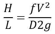
where:
The Darcy Weisbach equation is dimensionally correct for any consistent set of units, such as metric (SI) or imperial, and applies to conduits of any shape.
Estimation of the friction factor f depends on the nature of the flow. Flow may be laminar or turbulent, and within the turbulent flow regime, may be ‘smooth’ turbulent or ‘rough’ turbulent. The flow regime is characterised by the Reynolds number (2) (dimensionless):
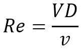
where:
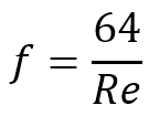
Laminar flow, also known as viscous or streamline flow occurs at low velocities in small bore conduits, or with fluids of higher viscosity. Friction losses are controlled by shearing resistance between layers of fluid. Under this flow regime, the friction factor is controlled entirely by viscous shear (3):
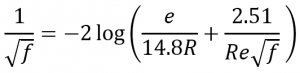
Laminar flow is characterised by purely axial movement of fluid particles. As the velocity increases, flow becomes unstable and turbulence develops, with fluid particles having a lateral velocity component, markedly increasing energy losses. Initially, viscous influences predominate. With further velocity increase, the roughness of the conduit surface start to influence the losses, and at very high velocity, this becomes the controlling factor. Most practical flow situations lie in the “transition” zone, where the friction factor is governed partly by viscous effects and partly by surface roughness. The predictive equation used is the Colebrook-White function (4):
The flow regime is characterised by the Reynolds number, Re. The change from laminar to turbulent flow occurs between Re = 2000 – 4000 depending on the surface roughness. In this range, there is some uncertainty as to the flow regime that will apply.
Equations (1), (2) and (3) for laminar flow and (1), (2) and (4) for turbulent flow can be combined into a single equation for flow velocity, noting that:
Q = AV
where:
The solution is trivial for laminar flow for any of the variables. For turbulent flow direct solution is only possible for V. For other variables a trial and error solution is obtained using an iterative approach.
The cross-over region between laminar and turbulent flow is handled by averaging the velocity as computed by both methods. This is considered to apply when a condition is determined such that simultaneously the Reynolds number for the turbulent regime is less than 2000, and the Reynolds number for the laminar regime is greater than 2000.
Other Flow Formulas
When solving the Darcy Weisbach equation for the velocity of the flow V the solution is complicated by the fact that friction factor f is itself a function of V. Empirical equations have been established to attempt to simplify the solution. Examples include the Hazen-Williams formula and the Manning formula. These empirical formulas are not applicable to all flows and introduce an error of unknown magnitude. In FLUFF calculations the equivalent Hazen Williams coefficient and Mannings’s number are calculated and displayed on the screen.
Roughness Coefficients
The roughness coefficients incorporated in FLUFF as default values are the smoothest values given in Australian Standard 2200 and are for clean concentrically jointed pipes. The coefficient may need to be varied depending on biological or slime growths, mineral deposits, corrosion, erosion or air entrapment. It is the responsibility of the user to ensure correct engineering judgement is used in selecting a coefficient appropriate to the application.
Form Resistance to Flow
In a pipeline, energy is lost wherever there is a change in cross-section or flow direction. These energy losses which occur as a result of disturbances to the normal flow show up as pressure drops in the pipeline.
These “form losses” which occur at sudden changes in section, at valves and at fittings are usually small compared with the friction losses in long pipelines. However, they may contribute a significant part to the total losses in short pipeline systems with several fittings. FLUFF does not deal with form losses. However, some background information is given below.
It can be shown that form losses in pipes may be expressed as a constant multiplied by the velocity head:
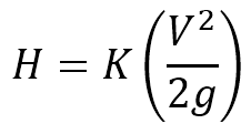
where:
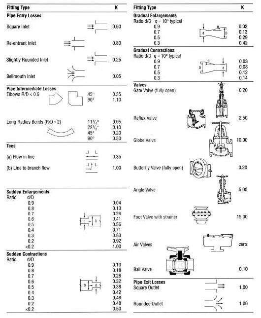
For any pipeline system the total form resistance to flow can be determined by adding together the individual head losses at each valve, fitting or change in cross section.
Data Entry
Pipe material: select from a wide variety of pre-defined pipe materials. The selection of a particular material from the drop-down list causes the program to load appropriate default values for all data entry fields.
Design stress: defaults to the standard value for the material selected.
Roughness (Hydraulic): defaults to the smoothest values given in Australian Standard 2200, but may be overwritten by entering the average roughness (in mm) of the internal pipe surface.
Standard Pipe or Cross section Type: select either a standard pipe or the type of cross-section (circular, square etc.) of the pipe.
- If a standard pipe is selected then select the standard used in manufacturing the pipe from the list of standards. The selection will load both the nominal pipe size and default class. The nominal size may be modified, as may the class.
- If a cross-section is selected then select the type and dimensions of the cross-section.
Length of pipe or cross-section: enter the length of the pipe (in m). This will result in recalculation holding the last entered two primary variables constant. The default length is 100m, so that the head loss reported is normally the percent hydraulic gradient.
Viscosity: enter the hydraulic viscosity multiplied by 1E-6 (in m2/sec or ft2/sec). For water and air, the program contains functions which estimate the viscosity as a function of temperature.
- Temperature: select air or water, and enter the temperature thereof. The viscosity is calculated and displayed.
Note: Predicted values for water and air are based on best fit equations of data from several published sources. For water the data spans the range 0-100 deg C, and extrapolation outside of this range is not permitted by the program. For air, the data spans the range -18 to 94 deg C, and although the program will allow extrapolation, the validity is unknown and caution should be exercised.
Flow Rate: enter the desired flow rate (in litres/sec or ft3/sec).
Velocity: enter the desired velocity (in m/sec or ft/sec).
Head Loss: enter the desired head loss (in m or ft).
Operation
The primary variables are the hydraulic mean radius D, (calculated from the cross-section and dimensions), flow rate F, velocity V and head loss H. Solution is possible for any two of these variables given the other two. When computing these variables, the most recently entered two variables are regarded as the “given” variables, and are held constant while the other two are recalculated. The two held variables are indicated by the pink background colour. Thus, if for example D is selected and then F is set, then V and H will be calculated, and will be recalculated for any changes in other variables, until either V or H is entered. If V is entered, for example, D and H will be calculated. If H is subsequently entered then F and D will be calculated. This sometimes leads to an unexpected response from the program, if consideration is not given to the order in which variables are entered.
During the calculations, the specified class is held constant. Occasionally, if the entered variables require recalculation of D and there is no pipe of that size and pressure class in the database, the following error message will be displayed: “Value out of bounds for this pipe size” Select an alternative class or reconsider the variables to continue.
Recomputation is executed each time a value is changed. In general an attempt will be made to interpret any entry to enable recomputation.
From a practical point of view it is redundant to provide solution systems for all possible permutations. Certain variables are therefore considered as constants, that is, although provision is made to allow them to be varied as input items, they cannot be calculated as a function of the other variables. These are E, L, and Y.
FLUFF is Copyright © 2006 Vinidex Pty Limited. All Rights Reserved.